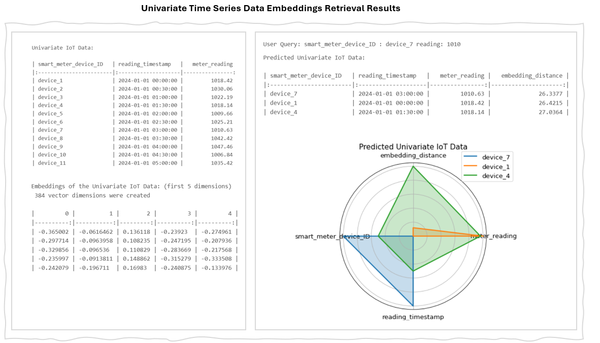
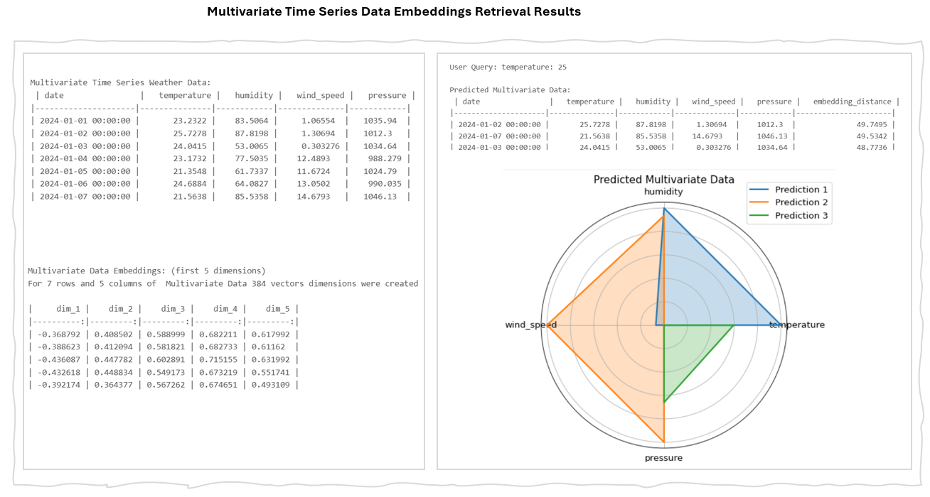
Text Objects
Word embeddings, sentence embeddings, and document embeddings are most common type of embedding techniques in natural language processing (NLP) for representing text as numerical vectors.
Word embeddings capture the semantic relationships between words, such as synonyms and antonyms, and their contextual usage. This makes them valuable for tasks like language translation, word similarity, synonym generation, sentiment analysis, and enhancing search relevance.
Sentence embeddings extend this concept to entire sentences, encapsulating their meaning and context. They are crucial for applications such as information retrieval, text categorization, and improving chatbot responses, as well as ensuring context retention in machine translation.
Document embeddings, similar to sentence embeddings, represent entire documents, capturing their content and general meaning. These are used in recommendation systems, information retrieval, clustering, and document classification.
Types of Text and Word Embedding Techniques
There are two main categories of word embedding
| Category | Description |
|---|---|
| 1. Frequency-Based Embedding | Frequency-Based embedding generate vector representations of words by analysing their occurrence rates in a given corpus. These approaches use statistical measures to capture semantic information, relying on how often words appear together to encode their meanings and relationships.
There are two types of Frequency-based embedding : |
| 2. Prediction-based embedding | Prediction-based embedding are created using models that learn to predict a word based on its neighbouring words within sentences. This approach focuses on placing words with similar contexts near each other in the embedding space, resulting in more nuanced word vectors that effectively capture a range of linguistic relationships.
There are three types of Prediction-based embedding : |
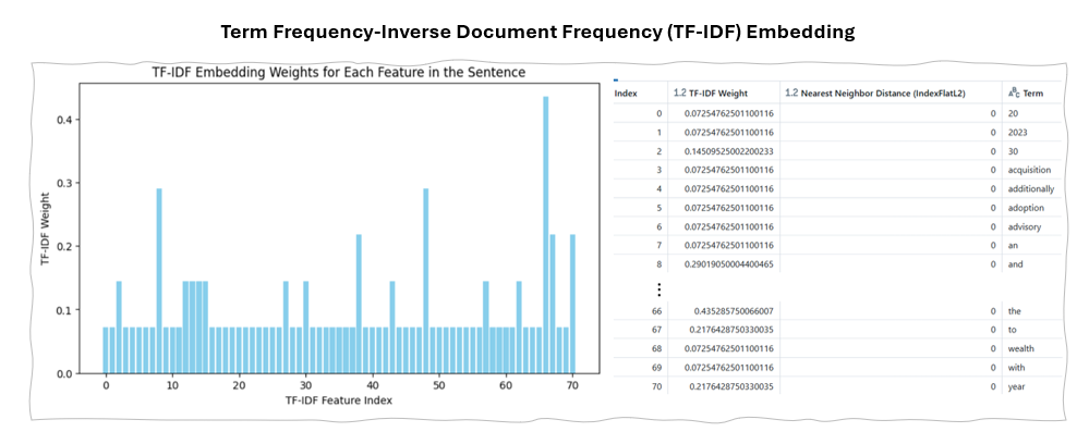
1.a. Term Frequency-Inverse Document Frequency (TF-IDF)
Is a basic embedding technique, where words are represented as vectors of their TF-IDF scores across multiple documents.
A TF-IDF vector is a sparse vector with one dimension per each unique word in the vocabulary. The value for an element in a vector is an occurrence count of the corresponding word in the sentence multiplied by a factor that is inversely proportional to the overall frequency of that word in the whole corpus.
Example Implementation of TF-IDF
Example of TF-IDF Embedding Result


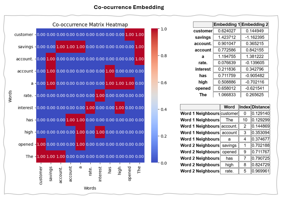
1.b Co-occurrence Matrix
A co-occurrence matrix quantifies how often words appear together in a given corpus, representing each word as a vector based on its co-occurrence frequencies with other words. This technique captures the semantic relationships between words, as those that frequently appear in similar contexts are likely to be related.
In essence, the matrix is square, with rows and columns representing words and cells containing numerical values that reflect the frequency of word pairs appearing together.
Example Implementation of Co-occurrence
Example of Co-occurrence Matrix Embedding Result
2 Prediction-Based Embedding
Prediction-based methods use models to predict words based on their context, producing dense vectors that place words with similar contexts close together in the embedding space.
2.a Word2Vec
Word2Vec transformed natural language processing by converting words into dense vector representations that capture their semantic relationships. It generates numerical vectors for each word based on their contextual features, allowing words used in similar contexts to be closely positioned in vector space. This means that words with similar meanings or contexts will have similar vector representations.
There are two main variants of Word2Vec
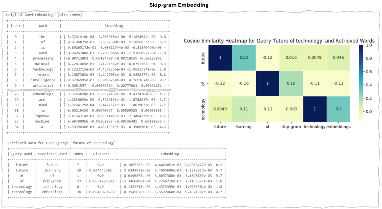
2.a.1 Skip-gram
Skip-gram is a method for generating word embeddings that predicts the surrounding words based on a specific "target word." By assessing its accuracy in predicting these context words, skip-gram produces a numerical representation that effectively captures the target word's meaning and context.
This approach is particularly effective for less frequent words, as it emphasizes the relationship between each target word and its context, enabling a richer understanding of semantic connections.
Example Implementation of Skip-gram
Example of Skip-gram Result
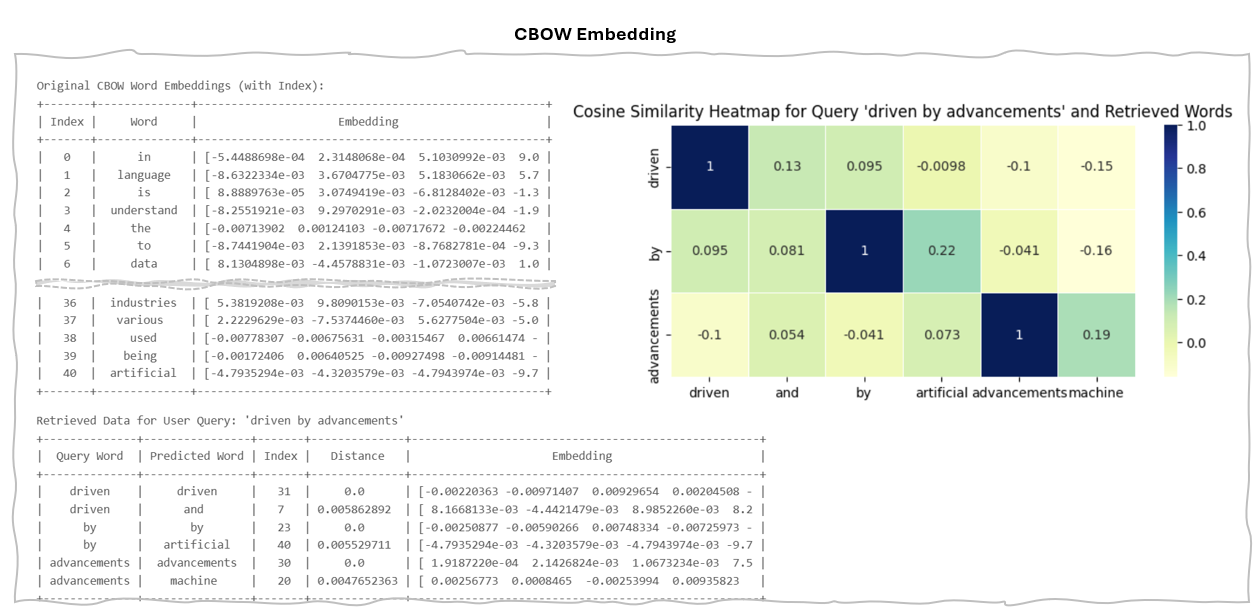
2.b.1 Continuous Bag of Words (CBOW)
The Continuous Bag of Words (CBOW) model aims to predict a target word based on its surrounding context words in a sentence. This approach differs from the skip-gram model, which predicts context words given a specific target word. CBOW generally performs better with common words, as it averages over the entire context, leading to faster training.
Example Implementation of Continuous Bag of Words
Example of Continuous Bag of Words
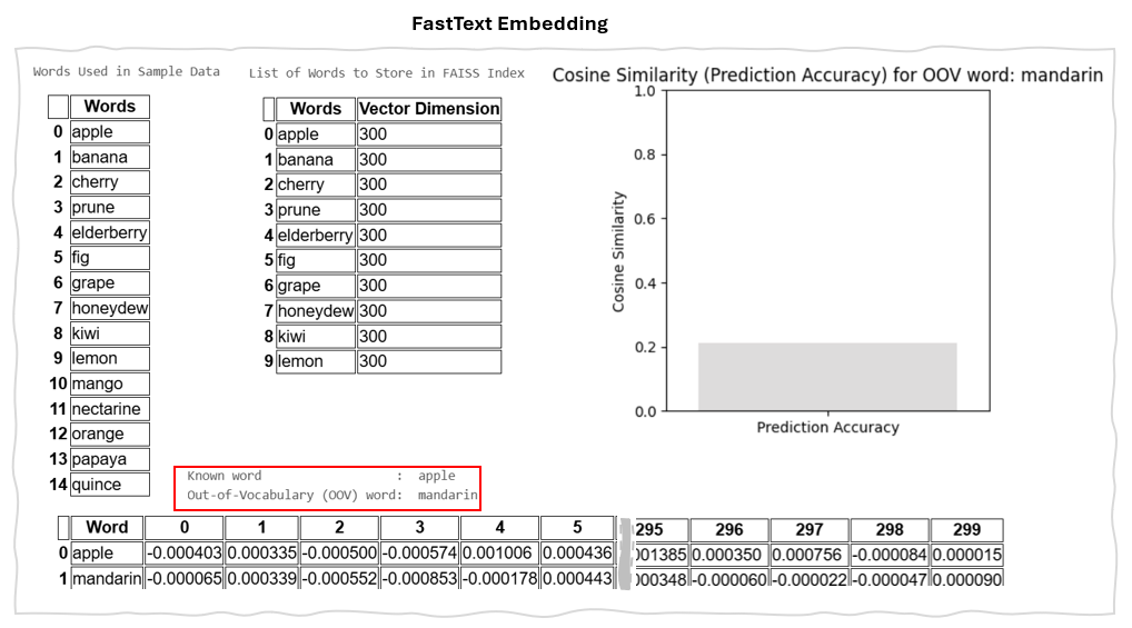
2.2 FastText
FastText embedding utilizes sub-word embeddings, which means it decomposes words into smaller components known as character n-grams, rather than treating them as single entities. This approach allows FastText to effectively capture the semantic meanings of morphologically related words. Additionally, because of its use of sub-word embeddings, FastText can manage Out-of-Vocabulary (OOV) words—those not included in the training data. By breaking down these words into sub-word units, FastText can generate embeddings even for terms absent from its initial vocabulary.
Example Implementation of FastText
Example of FastText Embedding Result
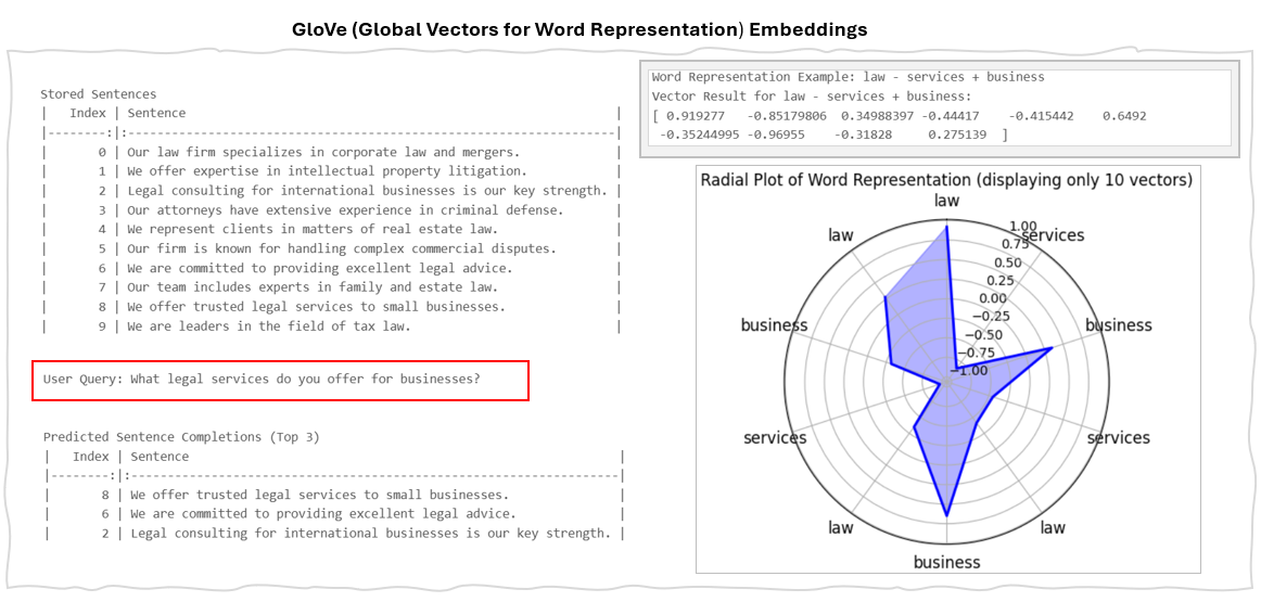
2.3 GloVe (Global Vectors for Word Representation)
GloVe embeddings are a type of word representation that capture the relationship between words by encoding the ratio of their co-occurrence probabilities as vector differences. The GloVe model learns these embeddings by analysing how often words appear together in a large text corpus. Unlike word2vec, which is a predictive deep learning model, GloVe operates as a count-based model.
It utilizes matrix factorization techniques applied to a word-context co-occurrence matrix. This matrix is constructed by counting how frequently each "context" word appears alongside a "target" word. GloVe then employs least squares regression to factorize this matrix, resulting in a lower-dimensional representation of the word vectors.
Example of GloVe Code
Example of FastText Embedding Result